
Understanding the Multilayer Perceptron (MLP)
1. Fernanda is no longer working alone
At the end of Article 3, Fernanda had built something rather useful: A little numerical decision-maker called a Threshold Logic Unit (TLU). It received Bedrooms and Location Code, combined them using weights and a bias, and returned YES or NO.
All very nice. But now Fernanda has a new problem. Some sellers do not want another YES or NO. Instead, they want an estimated price, preferably one that will not cause them to faint!
But hang on. We already tackled price prediction in Article 2. Fernanda combined Bedrooms and Location using a linear equation. Why complicate everybody’s afternoon by inviting Omar and Ricardo to the party?
Good point! However, consider a limitation of that earlier approach. In particular, recall that it adds a fixed amount for each bedroom, whether the house is in a Standard or a Prime location. Suppose, however, the historical pattern were different. Perhaps one extra bedroom is associated with an additional $30,000 in Standard locations but $70,000 in Prime locations. Then the effect of Bedrooms on the prediction depends on Location too. So, in this case, one fixed Bedroom Weight cannot represent both increases. Oh boy, what do we do now?
We could, of course, modify the original equation to include an additional calculation representing the interaction between Bedrooms and Location. That would be a perfectly reasonable approach. But what if we wanted a model that could learn useful combinations of its inputs without requiring us to specify every such interaction in advance?
This is where a different arrangement of calculations becomes interesting: Instead of passing Bedrooms and Location directly into one final price calculation, we could first let Omar and Ricardo process those inputs separately, using different numerical settings. Each would produce an intermediate response. Fernanda would then combine their responses to estimate the price.
The interesting possibility is that these intermediate responses, particularly when produced using nonlinear transformations, can allow the overall model to represent more complex relationships that our original linear calculation could not.
Sounds neat! But does that guarantee a better prediction? Not at all! However, the new approach does give us a more flexible way to reach a reasonable prediction.
And that, rather than simply providing employment opportunities for Omar and Ricardo, is why we are bringing them into the picture😊.
Let’s set the expectation here: We want to see how the team (Fernanda, Omar and Ricardo) produces a prediction. We note that a more flexible model is not necessarily a more accurate one. Whether the team can learn better settings from its mistakes is the subject of Article 5 so, hold your horses until then and let’s just concentrate on this article first!
For the remainder of this article the main question is:
What changes when Omar and Ricardo process the same property information, then Fernanda combines what they send her?
2. Thankfully, the same six houses are still here
We are keeping Properties A to F from Articles 1, 2 and 3 (see Table 1 below). There is no need to invent six new houses simply to give our three agents something to do. The location codes remain Standard = 0 and Prime = 1.
| Property | Bedrooms | Location | Location Code | Actual Sale Price |
|---|---|---|---|---|
| A | 2 | Standard | 0 | $200,000 |
| B | 3 | Standard | 0 | $250,000 |
| C | 4 | Standard | 0 | $280,000 |
| D | 2 | Prime | 1 | $300,000 |
| E | 3 | Prime | 1 | $400,000 |
| F | 4 | Prime | 1 | $450,000 |
The inputs are still Bedrooms and Location Code. The output we now want is a predicted sale price. Actual sale prices are known only because these six houses have already sold. Remember that we do not feed their actual prices into the prediction.
NOTE: For easier arithmetic, this article measures money in units of $100,000. Thus $300,000 becomes 3. Article 2 used $10,000 units. We are changing the measuring unit, not the houses or their prices. We will convert back to dollars whenever the result needs to look like a house price.
3. Who tells whom what?
Imagine Omar and Ricardo sitting at two desks. Both receive exactly the same two facts about a property: Its number of bedrooms and whether the location is Standard or Prime.
Each makes a separate calculation. Each sends one numerical response to Fernanda. Fernanda receives those two responses and combines them into the final price estimate. In our deliberately specified network, she does not receive the original bedroom count or location code directly.
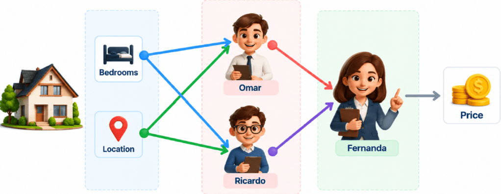
Notice that information moves in one direction while the prediction is made:
Inputs → Omar and Ricardo → Fernanda → Predicted Price
We will shortly give that movement its technical name. Just wait a few seconds, OK?
4. Omar and Ricardo have different settings
Each junior (that is how we refer to Omar and Ricardo individually with their boss, Fernanda, being the senior) has two weights and one bias, just as the TLU in Article 3 had weights and a bias. But here is the beauty of this extra layer of estate agents (who said being a junior is not a big deal!): The two juniors need not use the same settings! In fact, for our first attempt, let’s choose the values as in Table 2 below:
| Agent | Bedroom Weight | Location Weight | Bias |
|---|---|---|---|
| Omar | 2 | 1 | −4 |
| Ricardo | 1 | 3 | −3 |
So, Omar calculates his score as Score = (2 × Bedrooms) + (1 × Location Code) − 4, while Ricardo calculates his score as Score = (1 × Bedrooms) + (3 × Location Code) − 3.
Now let’s compare the 2 calculations:
Omar’s calculation is more responsive to one additional bedroom. Ricardo’s is more responsive to the change from Standard to Prime. It is important to note that what we just saw describes their numerical settings, not a discovery that a bedroom is more valuable than a location. In other words, these settings are initial values of weights and do not represent an underlying fact about the relative importance of Bedrooms and Location.
Their biases provide a fixed shift to each score. Because each junior has his own bias, the same property can produce different scores even before we decide what to pass on. This, my friends, is a sign of additional flexibility that the new approach offers us.
5. A score is not always the number we pass onward
Article 3 gave us a Step Function such that: Below the cutoff it returned 0, otherwise 1. This was useful for a YES/NO decision. Our juniors, however, need to send numerical information that can vary by more than one bit. That is to say, we need Omar and Ricardo to communicate more than a simple Yes/No (1 or 0). But how?
Suppose each junior follows this simple rule: If the score is negative, send 0, otherwise, send the score itself (see Table 3 below for some examples):
| Junior’s Score | Outgoing Response |
|---|---|
| −2 | 0 |
| −0.5 | 0 |
| 0 | 0 |
| 1 | 1 |
| 2 | 2 |
| 3.5 | 3.5 |
Now that we know what the rule does, we can name it: The Rectified Linear Unit (ReLU), a common Activation Function. We can write the ReLU function more formally as:
ReLU(z) = max(0, z)
An Activation Function transforms a unit’s score into the value sent onward. The Step Function from Article 3 was another Activation Function, but its output was restricted to 0 and 1. You see how easy it is to learn seemingly complex terminology? You just need to wait a bit and carefully listen to me!
Anyway, ReLU is not a miniature estate agent exercising judgment. It is just the numerical rule described above. A negative score becomes zero, zero becomes zero, and a positive score passes through unchanged. Coooooool!
6. Fernanda combines the messages
Fernanda, being a senior agent and quite an independent individual, has her own adjustable settings. To start, she gives each colleague’s message a weight of 0.5 and adds a bias of 1. So, her calculation (similar to what we saw in Article 2) is:
Predicted Price Units = (0.5 × Omar’s Response) + (0.5 × Ricardo’s Response) + 1
Note that her output is a price number, so we use a linear output. This means we do not need a Step Function or a ReLU after her final sum. She simply returns the numerical result, which we multiply by $100,000 to get to the actual price prediction.
The bias of 1 corresponds to a starting contribution of $100,000 (remember that bias always means a shift in this situation). The two weights control how much each message (from Omar and Ricardo respectively) affects the prediction. Their initial sum (0.5 for Omar and o.5 for Ricardo) happens to be 1 in our example. However, the network does not require weights to sum to 1. Nor do they have to remain positive when learning begins.
7. One property, all the way through
Now, let’s choose Property D, our familiar two-bedroom Prime property. Its input values are Bedrooms = 2 and Location Code = 1. Its actual historical sale price is $300,000, or 3 units. Here we have:
Omar’s score: (2 × 2) + (1 × 1) − 4 = 1. Therefore ReLU(1) = 1, so Omar sends 1 as his score to Fernanda.
Ricardo’s score: (1 × 2) + (3 × 1) − 3 = 2. So ReLU(2) = 2, so Ricardo sends 2 as his score to Fernanda.
Fernanda’s prediction: (0.5 × 1) + (0.5 × 2) + 1 = 2.5 units which, in dollars, is $250,000.
Let’s be precise then: $250,000 is a prediction; $300,000 is what Property D actually sold for. The prediction is $50,000 too low. The network has performed every calculation correctly so, why we are short of $50,000 in our prediction? Well, because the network’s chosen settings are simply not yet good enough. In other words, it still has some “learning” to do!
8. Now do all six. No disappearing houses, please!
As before, the same weights and biases are applied to every property. Of course, the inputs change from house to house. But the parameters do not change during this first round of predictions.
| House | Omar: Score → Response | Ricardo: Score → Response | Fernanda: Predicted Units | Actual Units |
|---|---|---|---|---|
| A | 0 → 0 | −1 → 0 | 1.0 | 2.0 |
| B | 2 → 2 | 0 → 0 | 2.0 | 2.5 |
| C | 4 → 4 | 1 → 1 | 3.5 | 2.8 |
| D | 1 → 1 | 2 → 2 | 2.5 | 3.0 |
| E | 3 → 3 | 3 → 3 | 4.0 | 4.0 |
| F | 5 → 5 | 4 → 4 | 5.5 | 4.5 |
For example, House C has four bedrooms and a Standard location. So, we have:
Omar’s core before ReLU: (2 × 4) + (1 × 0) − 4 = 4. Therefore Omar’s score after ReLU: ReLU(4) = 4.
Ricardo’s core before ReLU: (1 × 4) + (3 × 0) − 3 = 1. Therefore Ricardo’s score after ReLU: ReLU(1) = 1.
Fernanda’s prediction: (0.5 × 4) + (0.5 × 1) + 1 = 3.5 units = $350,000. Note that the actual sale price was $280.000.
House E, meanwhile, is predicted exactly. Wonderful! Before we open the champagne, however, notice the other five houses. One lucky answer does not rescue an entire model.
Anyway, time for some useful terminology: The process of using current settings to move from inputs through the network to a prediction is called the forward pass and we have now completed it for all six properties.
9. Why bother with ReLU? Is this not just Linear Regression in a fancy suit?
This is a super important question so, well done for asking it!
The answer requires a bit of an effort on the reader’s side but I promise you that the answer is more interesting than the name “Rectified Linear Unit” might suggest! So, let me do this:
Let’s return to Omar, Ricardo and Fernanda, and use the numerical settings we introduced earlier in this article.
Remember that Omar and Ricardo each receive the same two inputs, Bedrooms and Location Code, but use different weights and biases to calculate their scores.
Their original calculations are as follows.
Omar:
- Bedroom Weight = 2
- Location Weight = 1
- Bias = −4
Therefore,
Omar’s Score = (2 × Bedrooms) + (1 × Location Code) − 4
Ricardo:
- Bedroom Weight = 1
- Location Weight = 3
- Bias = −3
Therefore,
Ricardo’s Score = (1 × Bedrooms) + (3 × Location Code) − 3
Fernanda then receives their responses and calculates the predicted price using her own settings.
Fernanda:
- Weight on Omar = 0.5
- Weight on Ricardo = 0.5
- Bias = 1
Her calculation is:
Predicted Price Units = (0.5 × Omar’s Response) + (0.5 × Ricardo’s Response) + 1
And remember that one price unit represents $100,000.
So far, nothing new. These are exactly the settings we have already used.
Now, let’s ask an interesting question:
What would happen if Omar and Ricardo did not apply ReLU to their scores?
In other words, suppose they simply passed their calculated scores directly to Fernanda, including negative scores, without converting them to zero.
In that case, Omar’s Response would simply equal Omar’s Score, and Ricardo’s Response would equal Ricardo’s Score.
We can therefore replace their responses in Fernanda’s equation with their original calculations. OK then. Let’s do exactly that:
Predicted Price Units = 0.5 × ((2 × Bedrooms) + (1 × Location Code) − 4) + 0.5 × ((1 × Bedrooms) + (3 × Location Code) − 3) + 1
Now look carefully at what happens to Predicted Price Units when we first multiply out the terms:
Predicted Price Units = (0.5 × (2 × Bedrooms)) + (0.5 × (1 × Location Code)) + (0.5 × -4) + (0.5 × (1 × Bedrooms)) + (0.5 × (3 × Location Code)) + (0.5 × -3) + 1
And continue reading to see what we get for Predicted Price Units when we change the position of some of the terms so that:
- Both entries for Bedrooms (Omar’s and Ricardo’s) are together,
- Both entries for Location Code (Omar’s and Ricardo’s) are together, and
- The three entries for Bias (Omar’s, Ricardo’s, and Fernanda’s) are together.
We end up with the following:
Predicted Price Units = (0.5 × (2 × Bedrooms)) + (0.5 × (1 × Bedrooms)) + (0.5 × (1 × Location Code)) + (0.5 × (3 × Location Code)) + (0.5 × -4) + (0.5 × -3) + 1
OK. We are almost there. Now, the total contributions from Bedrooms become:
(0.5 × 2 × Bedrooms) + (0.5 × 1 × Bedrooms)
= (1 + 0.5) × Bedrooms
= 1.5 × Bedrooms
Similarly, the total contributions from Location Code become:
(0.5 × 1 × Location Code) + (0.5 × 3 × Location Code)
= (0.5 + 1.5) × Location Code
= 2 × Location Code
And finally, the three constant values, representing the biases, combine to give us the following:
(0.5 × −4) + (0.5 × −3) + 1
= − 2 − 1.5 + 1
= −2.5
Phew! Putting everything together, Fernanda’s entire three-agent calculation becomes:
Predicted Price Units = (1.5 × Bedrooms) + (2 × Location Code) + (-2.5) or more simply:
Predicted Price Units = (1.5 × Bedrooms) + (2 × Location Code) – 2.5
Notice something rather surprising in the above equation: We started with three agents, each using their own weights and biases independently. Yet, after combining their calculations, we ended up with exactly the same general structure we encountered in Article 2. “What is the general structure?” I hear you ask. Well, this is the structure that includes a weighted contribution from Bedrooms, plus a weighted contribution from Location, plus a starting amount (bias)!
WHAAAAAT? Are you serious?
Yes, please relax, and don’t panic on me just yet! Let’s verify this using Property D, our familiar two-bedroom property in a Prime location to see what is happening.
For Property D we have:
- Bedrooms = 2
- Location Code = 1
So, using the simplified equation we get:
Predicted Price Units = (1.5 × 2) + (2 × 1) − 2.5
= 3 + 2 − 2.5
= 2.5 units, or $250,000
We can also obtain exactly the same result by calculating the agents’ responses separately, without ReLU.
Omar’s Score = (2 × 2) + (1 × 1) − 4 = 1
Ricardo’s Score = (1 × 2) + (3 × 1) − 3 = 2
Fernanda’s Prediction = (0.5 × 1) + (0.5 × 2) + 1 = 2.5 units, or $250,000
The two approaches produce identical results! Darn! Why should anyone care if both approaches produce the same result? In fact, is there any point to this line of reasoning?
Yes, there is. Because there is an important detail worth noticing here: For Property D, both Omar and Ricardo already produced positive scores (1 and 2 respectively). ReLU would therefore leave their responses unchanged anyway.
But, the difference between the two approaches becomes visible when a score is negative.
Aha! And here is how:
Consider Property A, our two-bedroom property in a Standard location.
Omar’s Score = (2 × 2) + (1 × 0) − 4 = 0
Ricardo’s Score = (1 × 2) + (3 × 0) − 3 = −1
Without ReLU, Ricardo sends −1 to Fernanda. So, we will get:
Fernanda’s Prediction = (0.5 × 0) + (0.5 × −1) + 1 = 0.5 units, or $50,000.
But with ReLU, Ricardo’s negative score becomes zero, and we get:
Fernanda’s Prediction = (0.5 × 0) + (0.5 × 0) + 1 = 1 unit, or $100,000.
So:
The prediction has changed, even though every weight and bias remains exactly the same!
And here lies the important distinction:
Without ReLU (or any other nonlinear activation function), our three-agent network is mathematically equivalent to a single linear calculation of the original inputs. So, simply adding more agents and more layers of weighted sums would not change that fundamental limitation of our original model.
With ReLU, however, something important changes: Instead of passing their calculated scores directly to Fernanda, Omar and Ricardo replace any negative score with zero while leaving positive scores unchanged. This allows the network to respond differently to changes in the original inputs, depending on whether an intermediate score is positive or negative. As a result, the network can represent relationships that a single linear calculation cannot.
Figure 2 below shows the prices predicted by our three-agent network for Standard and Prime properties with two, three and four bedrooms using ReLU.
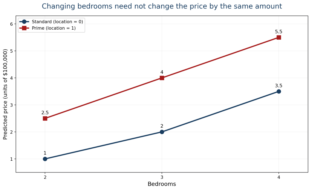
Look closely at the Standard properties in Figure 2. We see that:
- With two bedrooms, the predicted price is 1 unit ($100,000),
- With three bedrooms, the predicted price is 2 units ($200,000),
- With four bedrooms, the predicted price is 3.5 units ($350,000).
Notice what happens when we add one bedroom:
- Moving from two to three bedrooms increases the prediction by 1 unit (2 – 1), which is equivalent to $100,000,
- But moving from three to four bedrooms increases it by 1.5 units (3.5 – 2), or $150,000.
Why the difference?
Because Ricardo’s score is negative for the two-bedroom Standard property (-1), zero for the three-bedroom property (0), and positive for the four-bedroom property (1). ReLU, therefore, blocks his negative score (equivalent to passing zero), passes zero when the score is zero, and passes his positive score, unchanged, onward. This changes how the network responds as the number of bedrooms increases.
Our original linear model in Article 2, using separate contributions from Bedrooms and Location, would always assign the same additional amount to one more bedroom, provided Location remained unchanged.
This is why ReLU matters. It allows the network to capture relationships that our earlier linear model could not represent.
Does this mean our three-agent network is necessarily a better price predictor? Not at all! As we saw in Table 4, its current predictions are rather poor😞. What we have gained is greater flexibility, not guaranteed accuracy.
And now that we understand why combining several artificial neurons can be useful, we are ready to give this arrangement its proper technical name…
10. Let’s give the team its technical name
The structure we have constructed is called a Multilayer Perceptron (MLP), a type of feedforward artificial neural network. Our particular network has two numerical inputs, one hidden layer containing two artificial neurons, and an output layer containing one artificial neuron.
“Hidden” does not mean mysterious or inaccessible. It simply means these two units are between the input and the final output. Omar and Ricardo each produce an intermediate response while Fernanda produces the final prediction.
| Our Estate-Agency Story | What the Actual Network Does |
|---|---|
| Bedrooms and Location Code arrive | Receives two numerical inputs |
| Omar and Ricardo each examine the property and calculate a score | Two hidden neurons each calculate a weighted sum + bias, then apply ReLU |
| Each junior sends Fernanda one message | Two numerical hidden outputs become inputs to the output neuron |
| Fernanda combines their messages | Output neuron computes its weighted sum + bias |
| Fernanda states a price estimate | Network produces one numerical prediction |
A useful count: Omar has 3 parameters (two weights, one bias), Ricardo has 3 (two weights, one bias), and Fernanda has 3 (two incoming weights, one bias). That makes 9 adjustable parameters in our tiny network. The number of properties and their bedroom counts are inputs, not parameters.
For readers comfortable with notation, let x₁ be Bedrooms and x₂ be Location Code. Also, let O represent Omar’s score, R represent Ricardo’s score and ŷ represent Fernanda’s final prediction. Then:
O = ReLU(2x₁ + x₂ − 4)
R = ReLU(x₁ + 3x₂ − 3)
ŷ = 0.5 O + 0.5 R + 1, with ŷ measured in $100,000 units
Those symbols describe exactly what we have already calculated. No new magic has been smuggled in. However, you may probably look smarter amongst your friends if you wrote the calculations using these symbols instead😊.
11. Building the network is necessary for this approach, but it is not enough
We now have an MLP: Information flows through two intermediate neurons and reaches a final neuron, which predicts a price. This is an essential step toward understanding neural networks. Nice!
But the network does not improve itself merely because the three agents are cooperating. All nine settings were supplied by us. The model has not yet “learned” from the six historical sale prices.
Look at Property D again. $250,000 predicted against $300,000 of actual price. We could raise Fernanda’s bias, increase her weight on Ricardo, change Omar’s bedroom weight, or adjust several settings together. Each choice affects the prediction differently, and because the same parameters serve all six houses, improving D could make another house worse.
So which setting should change, in which direction, and by how much? That is not a question the forward pass can answer. We need a way to measure the mistake and trace how each setting contributes to it.
12. Question time
- Why do Omar and Ricardo receive the same two property inputs but produce different messages?
- What does ReLU send onward when its input is −1? What about 2?
- For Property D, reproduce the values 1, 2 and 2.5.
- Why is Fernanda’s final unit linear rather than a Step Function?
- If all activations were linear, what kind of calculation would the whole network reduce to?
- How many adjustable parameters does this MLP contain?
- Does an accurate forward calculation guarantee an accurate prediction?
13. What have we learned?
We have progressed from one TLU to a network of three artificial neurons. We kept the same two property inputs and the same six houses, but changed how those inputs are processed. Omar and Ricardo create intermediate numerical responses, Fernanda combines them into a price. ReLU introduces nonlinear behavior, allowing the network to represent relationships beyond a single straight-line model. The forward pass tells us what the network predicts using its current settings.
What it does not tell us is how to improve those settings. An architecture that can make predictions is necessary but not sufficient for learning. That brings us to Article 5.
14. Next: The estimate was wrong. What should the team change?
Property D is still staring at us: The team estimated $250,000 for a house that sold for $300,000. There are nine settings it could change, and guessing is not a particularly reassuring training strategy. In our next article, we will introduce loss, gradients, backpropagation and gradient descent, beginning with intuition and then mathematics, and follow one learning step from beginning to end.
15. Question time: Suggested answers
- Because the agents use different weights and biases.
- ReLU(−1) = 0, ReLU(2) = 2.
- Omar: ReLU((2 × 2) + (1 × 1) − 4) = 1, Ricardo: ReLU((1 × 2) + (3 × 1) − 3 = 2) = 2, Fernanda: (0.5 × 1) + (0.5 × 2) + 1 = 2.5.
- We want a numerical price, rather than only 1 or 0 (yes or no).
- A single linear calculation of the original inputs, using weights and a bias, just like the model we introduced in Article 2.
- Nine: Three in each of three neurons.
- No. The calculations can be correct while the chosen parameter values produce a poor prediction.
Feedback please
I welcome your questions, corrections and suggestions. In particular, which part of the move from one neuron to several was least obvious?
NEXT ARTICLE
The Estimate Was Wrong. What Should the Team Change?
Understanding Loss, Gradients and Backpropagation

