Article 3 of 24: How Does an Estate Agent Make a Yes-or-No Decision?

Understanding the Threshold Logic Unit (TLU)

1. Why are we back to YES or NO?

What? “You must be joking”, I hear you say! Sadly, I am not.

At the end of Article 2, Fernanda had finally learned how to combine information about a property to produce something much more satisfying than YES or NO (an actual predicted sale price).

So why on earth are we going backwards?

Well, we are actually not! The question we are about to ask may be familiar, but the way we answer it will be different.

Back in Article 1, Fernanda had to decide whether a property belonged in the agency’s $300,000-and-above category:

Is this property expected to sell for at least $300,000: YES or NO?

There, we gave the computer several complete YES/NO rules and asked it to use historical examples to choose the one that worked best.

Then, in Article 2, we changed the task. Instead of choosing among complete rules, Fernanda learned how numerical information about a property could be combined to predict an actual sale price.

And now we are deliberately returning to the YES/NO question.

Couldn’t we simply take the price predicted in Article 2 and check whether it is at least $300,000?

Absolutely:-). And for our little property example, that would be perfectly reasonable. We do not actually need a new mechanism merely to answer this particular question.

But many real problems ask directly for a decision rather than for a numerical quantity first. For example:

• Approve or reject,
• Fraud or legitimate,
• Spam or not spam,
• Disease detected or not detected,
• YES or NO.

In such cases, it can be useful to build the decision directly from the available inputs.

That is what we are going to explore here. In other words, instead of first predicting a price, we will let the available property information contribute to a numerical score, and then use that score to decide whether the answer should be YES or NO.

Admittedly, there is also another reason for taking this apparent detour: This simple mechanism turns out to be an important stepping stone toward something much more powerful: The artificial neuron and, eventually, Neural Networks. Yupee!

So, we are not returning to YES/NO because Article 1 failed. We are returning to it because we are now ready to understand a different mechanism for producing that decision. That is to say we are aiming for:

Same question, new mechanism

2. Let us keep the same six houses

There is no need to invent another housing market simply because we have started another article. So, we will continue using the same six historical properties that accompanied Fernanda through Article 1 and Article 2 (see Table 1 below).

Property	Bedrooms	Location	Actual Sale Price	Correct Category
A	2	Standard	$200,000	NO
B	3	Standard	$250,000	NO
C	4	Standard	$280,000	NO
D	2	Prime	$300,000	YES
E	3	Prime	$400,000	YES
F	4	Prime	$450,000	YES

As before:

• NO means the property sold for less than $300,000,
• YES means the property sold for $300,000 or more.

The Actual Sale Price is useful because these are historical properties, meaning we already know what actually happened. In contrast, when a new property arrives, its eventual sale price is not yet known.

Fernanda therefore needs to use the information she does have about that property to produce a prediction. And once again, for our deliberately simplified little world, she has only two pieces of information:

• Number of Bedrooms
• Location

So the difference this time is not the data, but is what we are going to do with it.

3. What information does Fernanda already have?

Fortunately, Fernanda is not starting from scratch. If you recall, in Article 2, we already saw that the two inputs do not arrive in quite the same form:

Bedrooms is already numerical. A house may have 2, 3 or 4 bedrooms, so that input is ready to take part in a calculation.

Location, however, arrives as a category:

• Standard
• Prime

In Article 2, we gave those two possibilities a simple numerical representation (see Table 2 below):

Location	Location Code
Standard	0
Prime	1

Remember that this does not mean Standard is “worth zero” while Prime is “worth one”! The numbers simply provide a convenient numerical way to distinguish the two possibilities.

We also learned something else important in Article 2: Different inputs can make different numerical contributions to a calculation, and those contributions can be controlled by adjustable numerical settings. Later, we gave those settings their usual Machine Learning name: Weights.

We also encountered another adjustable setting: Bias. So Fernanda already has several useful ingredients available:

• Numerical inputs,
• Weights that control how those inputs contribute to a calculation,
• And a bias that can shift the result.

But there is one important difference between Article 2 and the problem in front of us now; In Article 2, all those ingredients were combined to produce a predicted price. This time, however, Fernanda does not actually need a price. Instead, she needs a decision: YES or NO.

Can Fernanda use the same kind of numerical ingredients to produce one number that helps her make that decision?

4. From a predicted price to a score

In Article 2, Fernanda combined numerical contributions from Bedrooms and Location to produce something with an obvious real-world meaning: A predicted sale price.

This time, however, she does not need to produce a price. She merely needs enough numerical information to help her decide between NO and YES.

So Fernanda tries a slightly different idea: What if Bedrooms and Location each contribute to a single number, but instead of interpreting that number as dollars, she simply uses it as a score? The score would not itself be the final answer, though. It would simply summarize the contributions from the information available to her.

To keep our first attempt easy to follow, suppose Fernanda starts with these trial settings:

• Bedroom Weight = 1
• Location Weight = 4

Remember what these numbers mean: A Bedroom Weight of 1 means that each additional bedroom contributes 1 score unit, while a Location Weight of 4 means that moving from Standard, whose Location Code is 0, to Prime, whose Location Code is 1, contributes an additional 4 score units.

Note that these are simply trial settings. We are not claiming that Location is somehow “four times more important” than Bedrooms in the real housing market!

Armed with these values, Fernanda can now calculate the following:

Score = (1 × Bedrooms) + (4 × Location Code)

Let us see what happens to our six historical properties (see Table 3 below):

Property	Bedrooms	Location Code	Score Calculation	Score	Correct Category
A	2	0	(1 × 2) + (4 × 0)	2	NO
B	3	0	(1 × 3) + (4 × 0)	3	NO
C	4	0	(1 × 4) + (4 × 0)	4	NO
D	2	1	(1 × 2) + (4 × 1)	6	YES
E	3	1	(1 × 3) + (4 × 1)	7	YES
F	4	1	(1 × 4) + (4 × 1)	8	YES

Fernanda has therefore transformed the six properties into the following sequence of scores:

2, 3, 4, 6, 7, 8

A warning is useful here: A score of 8 does not mean $80,000, $800,000 or an 80% probability of anything. At this stage, the score is simply an internal numerical value produced from the inputs. Its usefulness will depend on what Fernanda does with it next.

5. A score is useful, but it is not yet a decision

Fernanda now has six scores. Very, very nice!

Unfortunately, none of her clients has asked: “Fernanda, what is my score?” Nope. They want an answer in an all-or-nothing kind of way: YES or NO.

So Fernanda needs another rule that turns the score into a decision. Look again at the historical examples (see Table 4 below):

Correct Category	Scores
NO	2, 3, 4
YES	6, 7, 8

Something rather convenient has happened, has it not? All the historical NO examples have scores of 4 or below, while all the historical YES examples have scores of 6 or above. Hmmm, interesting.

There is, therefore, a gap between the two groups. This means that Fernanda could place a dividing point (a cutoff, shall we say) somewhere inside that gap. For convenience, let us choose:

Cutoff = 5

Then her decision rule becomes:

• If Score < 5 → Predict NO
• If Score ≥ 5 → Predict YES

That dividing value has a standard technical name: Threshold. So our cutoff of 5 is also the decision threshold.

The idea itself is wonderfully simple:

Calculate a score, compare it with a threshold, and let that comparison determine the answer

6. Let us see whether the decision rule actually works

We can now apply Fernanda’s new rule to all six historical houses (see Table 5 below).

Remember:

• Score < 5 → NO
• Score ≥ 5 → YES

Property	Score	Decision Using Threshold 5	Correct Category	Result
A	2	NO	NO	Correct
B	3	NO	NO	Correct
C	4	NO	NO	Correct
D	6	YES	YES	Correct
E	7	YES	YES	Correct
F	8	YES	YES	Correct

Well, that went suspiciously well! For our deliberately simple historical examples, Fernanda’s trial weights together with a threshold of 5 classify all six properties correctly. Aren’t we lucky!

But let us concentrate on the mechanism rather than congratulate Fernanda too enthusiastically.

She performed two distinct operations:

First: Calculate

She combined the inputs to produce a numerical score.

Second: Decide

She compared that score with a threshold and produced either NO or YES.

We can write the second operation very simply:

• Score below threshold → 0
• Score at or above threshold → 1

where:

• 0 represents NO
• 1 represents YES

A rule that changes its output from one value to another when a threshold is crossed is commonly called a Step Function.

Again, the name is less important than the mechanism. We already understood what the rule did before learning what it was called!

7. But what happened to the bias?

You may have noticed something slightly odd.

In Article 2, bias played an important role in our calculation.

Yet so far in this article, Fernanda has used:

• Bedroom Weight,
• Location Weight,
• And a threshold,

but no bias.

Has bias mysteriously disappeared? Nope. In fact, this gives us a useful opportunity to understand the relationship between bias and the threshold.

Our current scores are:

2, 3, 4, 6, 7, 8

and Fernanda compares them against a threshold of:

5

So she currently asks: Is the score at least 5?

But suppose instead that she subtracts 5 from every score (see Table 6 below):

Original Score	Subtract 5	New Score
2	−5	−3
3	−5	−2
4	−5	−1
6	−5	1
7	−5	2
8	−5	3

Now look what has happened: The NO examples have become: −3, −2, −1 while the YES examples have become: 1, 2, 3.

So, Fernanda no longer needs to compare them with a threshold of 5. She can simply ask:

• If Score < 0 → NO
• If Score ≥ 0 → YES

Nothing about the final classifications has changed. We have simply moved the scores rather than moving the threshold.

And how do we shift every score downward by 5? We add the same value, −5, to every score to get:

Score = (1 × Bedrooms) + (4 × Location Code) + (−5)

That final value, −5, is our bias.

So there are two equivalent ways of describing what Fernanda just did:

Version 1

Calculate the score without bias and compare it with a threshold of 5.

Version 2

Add a bias of −5 to the score and compare the result with a threshold of 0.

For our example, both produce exactly the same decisions.

This also gives us a more concrete way to understand the bias we first encountered in Article 2:

Bias shifts all the scores relative to the decision threshold.

Fernanda now has everything she needs:

• Numerical inputs,
• Weights,
• A bias,
• A score,
• A threshold,
• And a rule that turns the score into 0 or 1.

We have, without formally naming it yet, built something rather important.

8. We have just built a Threshold Logic Unit

A Threshold Logic Unit? What is that?

Let us pause for a moment and look at what Fernanda has actually constructed. She:

1. Receives numerical inputs,
2. Lets each input make a contribution controlled by a weight,
3. Adds those contributions together with a bias to produce a score,
4. Compares that score with a threshold,
5. Produces one of two possible outputs: 0 or 1.

That complete mechanism has a technical name:

Threshold Logic Unit

Or, rather mercifully for those of us who dislike unnecessarily long names:

TLU

So our simple property decision can now be written as:

Score = (Bedroom Weight × Bedrooms) + (Location Weight × Location Code) + Bias

Using our current settings:

• Bedroom Weight = 1
• Location Weight = 4
• Bias = −5

we have:

Score = (1 × Bedrooms) + (4 × Location Code) − 5

Then the TLU applies its decision rule:

• If Score < 0 → Output = 0
• If Score ≥ 0 → Output = 1

where:

• 0 means NO
• 1 means YES

For example, consider Property D:

• Bedrooms = 2
• Location Code = 1

The score is:

Score = (1 × 2) + (4 × 1) − 5 = 1

Since 1 is at or above the threshold of 0:

Output = 1 → YES

And that matches the known historical category for Property D.

Note that nothing magical has happened. The TLU has simply performed a numerical calculation and then applied a threshold-based decision rule. Easy, right?

Figure 1 below summarizes the entire mechanism in one picture.

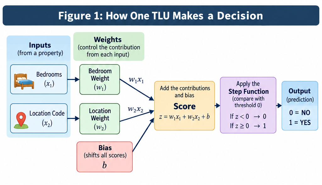
This is the basic mechanism we will eventually see again inside much larger Neural Networks.

9. Weights, bias and threshold do different jobs

Now that we have the complete mechanism in front of us, it is worth separating the roles of its three main numerical ingredients. They are related, but they do not do the same thing.

Weights control the contribution from each input:

Consider our score calculation:

Score = (1 × Bedrooms) + (4 × Location Code) − 5

The Bedroom Weight is 1. So increasing Bedrooms by one increases the score by 1, assuming everything else stays the same.

The Location Weight is 4. So moving from Standard (Location Code = 0) to Prime (Location Code = 1) increases the score by 4, assuming everything else stays the same.

The weights therefore control how strongly changes in each input affect the score.

But we should be careful with the word importance. A Location Weight of 4 and a Bedroom Weight of 1 do not automatically prove that Location is “four times more important” than Bedrooms in the real world.

The two inputs are represented on different numerical scales, and the weights belong to this particular model.

The weights control how each input contributes to the TLU’s score

Bias shifts every score:

Now consider the bias: Bias = −5. Before adding the bias, our six scores were: 2, 3, 4, 6, 7, 8.

After adding −5, they became: −3, −2, −1, 1, 2, 3. So, every score moved downward by exactly the same amount. That means something important:

Bias can shift the scores, but it cannot change their order

For example, before adding the bias: 2 < 3 < 4 < 6 < 7 < 8 and after adding the bias: −3 < −2 < −1 < 1 < 2 < 3. So, the order is unchanged.

This is one of the most useful distinctions to remember. If our weights arrange the properties in an unsuitable order, changing the bias alone cannot repair that problem.

The threshold decides where the output changes:

Finally, the threshold determines the point at which the TLU changes its output.

With our current convention:

• Score < 0 → 0
• Score ≥ 0 → 1

the threshold is 0.

So, the weights and bias produce the score, the threshold then decides what that score means for the final YES/NO decision.

A useful summary is:

• Weights shape the score,
• Bias shifts the score,
• Threshold turns the score into a decision.

That distinction will become increasingly important as our models become more complicated.

10. Why keep the threshold at zero?

At this point you might reasonably ask:

Why did we go to the trouble of moving all the scores by adding a bias? Why not simply keep the original scores and use a threshold of 5?

Excellent question!

And for this particular example, we absolutely could. In fact, these two approaches are equivalent:

Approach A

Use Score = (1 × Bedrooms) + (4 × Location Code) and compare the score with Threshold = 5.

Approach B

Use Score = (1 × Bedrooms) + (4 × Location Code) − 5 and compare the score with Threshold = 0.

Both produce exactly the same classifications for our six properties. So why is the second form useful?

Because keeping the decision threshold fixed at zero gives us a convenient standard form:

First calculate the score, including the bias. Then simply ask whether that score is below zero or at least zero.

That makes the mechanism easier to express consistently. And you know mathematicians: The just love consistency:-).

So, instead of moving the threshold around, we can let the bias absorb that shift. Pretty clever, right?

This is why you will often see simple threshold-based units written in the form:

Score = Input contributions + bias

followed by:

• Score < 0 → 0
• Score ≥ 0 → 1

It does not mean zero is somehow a naturally privileged decision point in the real world. We have simply chosen a convenient mathematical representation.

And that gives us another useful interpretation of bias:

Bias helps determine how much combined input evidence is needed before the TLU crosses the decision threshold.

At this stage, our chosen weights and bias happen to classify all six historical examples correctly.

But we should not get too comfortable. After all, we deliberately chose settings that make the mechanism easy to understand. But:

What happens when the TLU gets a prediction wrong?

11. What happens when the TLU gets one wrong?

So far, Fernanda has enjoyed suspiciously good luck. With Bedroom Weight = 1, Location Weight = 4 and Bias = −5, her TLU classified all six historical properties correctly.

But learning becomes much more interesting when the settings are not already perfect. So let us deliberately make Fernanda’s starting point a little worse.

Suppose she had instead started with:

• Bedroom Weight = 1
• Location Weight = 4
• Bias = −7

Her score calculation would then be:

Score = (1 × Bedrooms) + (4 × Location Code) − 7

Now consider Property D:

• Bedrooms = 2
• Location Code = 1
• Correct Category = YES

Fernanda calculates:

Score = (1 × 2) + (4 × 1) − 7 = −1

Since the score is below zero, the TLU predicts:

Output = 0 → NO

But the historical answer is:

Output = 1 → YES

So the prediction is wrong. Noooooooooooooo!

Let’s cool down a bit. This is exactly the kind of situation a learning procedure needs to respond to. Let’s see what we can do here.

In Article 2, we measured prediction error by comparing the actual value with the predicted value. We can use the same basic idea here.

The actual output is 1. The predicted output is 0. So:

Error = Actual Output − Predicted Output = 1 − 0 = +1

The positive error tells us something important:

The TLU produced 0 when it should have produced 1

In other words, for this example, the score needs to move upward enough to cross the threshold.

But knowing that a mistake occurred is only the beginning.

What should we change?

12. One small adjustment

Let us look at Property D again.

Its current score is −1. The threshold is 0.

So Fernanda does not need an enormous change. She merely needs the score to move from below zero to zero or above.

One simple way to do that is to increase the bias. Suppose Fernanda changes Bias = −7 to Bias = −6.

The weights remain unchanged.

Now she recalculates Property D:

Score = (1 × 2) + (4 × 1) − 6 = 0

And since Score ≥ 0, the TLU now produces:

Output = 1 → YES

The prediction has changed from wrong to correct. But we should check that Fernanda has not repaired one property by breaking all the others.

So, with the new bias of −6, the six scores become (see Table 7 below):

Property	Score	Prediction	Correct Category	Result
A	−4	NO	NO	Correct
B	−3	NO	NO	Correct
C	−2	NO	NO	Correct
D	0	YES	YES	Correct
E	1	YES	YES	Correct
F	2	YES	YES	Correct

So this particular adjustment works nicely for our six historical examples. Great!

But do not read too much into the fact that Fernanda found a useful new bias immediately.

We chose a deliberately simple example so that we could see what an adjustment actually does. A real learning procedure needs a consistent rule for deciding the following:

• Which setting or settings should change,
• In which direction,
• And by how much.

We are deliberately postponing that machinery here. Later in this series, we will return to the much deeper question of how learning procedures decide how numerical settings should change.

For now, the important idea is simpler:

A prediction error can provide information that helps a learning procedure adjust the TLU’s numerical settings

13. Did Fernanda really “learn” the right answer?

This is worth slowing down for:

Fernanda did not rewrite the whole decision mechanism after seeing one mistake. She kept the same general structure:

Inputs → Weighted contributions → Bias → Score → Threshold → Output

What changed was one numerical setting inside that structure:

Bias: −7 → −6

That distinction matters!

In Article 1, learning meant choosing among several complete YES/NO rules.

In Article 2, learning meant finding numerical settings inside a linear price-prediction model.

Here, learning can once again mean changing numerical settings. But this time inside a mechanism whose final output is a YES/NO decision.

So the basic pattern continues:

Keep the model structure, use historical examples to check its predictions, and adjust numerical settings when the predictions are not good enough

That does not mean Fernanda or the algorithm has somehow discovered everything worth knowing about housing.

People still decided:

• That the task was to predict whether a property belongs in the $300,000-and-above category,
• That Bedrooms and Location would be the available inputs,
• How Location would be represented numerically,
• That the decision mechanism would use a TLU,
• That the output would be represented as 0 or 1,
• And how the learning procedure would be allowed to adjust the model.

This is key so, remember it well:

The learning procedure works inside the possibilities we give it!

This is the same boundary we have been building throughout the series:

People specify the problem, available information and learning structure. The learning procedure uses examples to determine useful numerical settings within that structure.

And that prepares us for a useful question:

What, exactly, are the technical names for all the pieces we have now used?

14. Time to attach the technical names

We have now used nearly all the important pieces of a Threshold Logic Unit.

As usual in this series, we deliberately met the ideas before worrying too much about their technical names. So let us now tidy things up (see Table 8 below):

What We Have Been Using	Usual Technical Name
Bedrooms and Location Code	Inputs or Features
The numerical setting controlling each input’s contribution to the score	Weight
The value added to shift all scores	Bias
The number produced after combining the input contributions and bias	Score
The dividing point at which the decision changes	Threshold
The rule that converts the score into 0 or 1	Step Function
0 or 1 produced after applying the Step Function	Output or Prediction
The complete decision unit	Threshold Logic Unit (TLU)

None of these names introduces a new mechanism. We already know what each part does.

The terminology simply gives us a shorter and more standard way to talk about it.

There is one additional term worth introducing: The weights and bias are numerical values that can be adjusted during learning. Such adjustable numerical settings are commonly called:

Model Parameters

So, in our TLU:

• Bedroom Weight is a parameter,
• Location Weight is a parameter,
• Bias is a parameter.

The inputs are not parameters. They are the property information supplied to the TLU.

That distinction matters so, read this last passage again to make sure you are absolutely clear about that!

For Property D, for example:

• Bedrooms = 2 and Location Code = 1 are the inputs,
• Bedroom Weight = 1, Location Weight = 4 and Bias = −6 are the parameters.

The inputs can change from one property to another. The parameters describe the model we are currently using.

15. How mathematicians write the same mechanism

So far, we have deliberately written our calculations using descriptive names (well, apart from in Figure 1 above, when my mathematical past got the better of me!):

Score = (Bedroom Weight × Bedrooms) + (Location Weight × Location Code) + Bias

That makes the meaning easy to follow. But as we saw in Article 2, mathematicians and Machine Learning texts usually shorten such expressions using symbols.

Our two-input TLU score can be written as:

Score = w₁x₁ + w₂x₂ + b

where:

• x₁ is the first input,
• x₂ is the second input,
• w₁ is the weight attached to the first input,
• w₂ is the weight attached to the second input,
• b is the bias.

For our property example:

• x₁ = Bedrooms,
• x₂ = Location Code,
• w₁ = Bedroom Weight,
• w₂ = Location Weight.

Using the settings from our latest example:

• w₁ = 1,
• w₂ = 4,
• b = −6,

we have:

Score = (1 × Bedrooms) + (4 × Location Code) − 6

Then comes the second part of the TLU:

Output = Step(Score)

The Step Function simply applies the decision rule we already understand:

• If Score < 0 → Output = 0
• If Score ≥ 0 → Output = 1

So the compact mathematical version has not introduced anything new.

It has merely compressed the mechanism we have already built:

Inputs → Weights → Add contributions + Bias → Score → Step Function → Output

This is exactly the discipline we followed in Article 2:

Understand the mechanism first. Let notation save space later rather than create mystery.

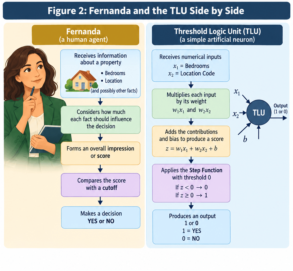
And now that both the mechanism and notation are in place, we are ready to put Fernanda and the TLU side by side.

16. Fernanda and the TLU side by side

By now, the resemblance between Fernanda’s reasoning and the TLU mechanism should be fairly clear.

Fernanda receives information about a property, gives different pieces of information different numerical influence, combines them into a score and then makes a YES/NO decision.

The TLU does the same kind of numerical work, without Fernanda’s experience, intuition or appreciation for suspiciously enthusiastic estate-agent descriptions!

We can now compare the two directly (see Table 9 below):

Fernanda	Threshold Logic Unit
Receives information about a property	Receives numerical inputs
Lets different facts contribute differently to the decision	Multiplies each input by its weight
Combines those contributions and a general shift	Adds the weighted contributions and bias
Obtains an overall impression or score	Produces a numerical score
Decides whether the score is enough for YES	Compares the score with the threshold
Says YES or NO	Produces 1 or 0

This comparison is useful, but we should keep one boundary very clear:

Fernanda understands what a bedroom is. She knows what a Prime location means. She has experience of buyers, neighborhoods and housing markets.

The TLU, on the other hand, understands none of those things. It receives numerical values and performs numerical calculations.

The human analogy explains the mechanism and illustrates the kind of numerical calculations the TLU performs. It does not mean that the TLU thinks like Fernanda. Remember that!

Figure 2 below places the two processes side by side:

17. Is a TLU already an artificial neuron?

We are now very close to terminology that appears throughout Neural Networks.

A TLU has:

• Inputs,
• Weights,
• A bias,
• A calculation that combines them,
• And a function that converts the resulting score into an output.

That structure should begin to look familiar if you have ever seen a diagram of an artificial neuron. And there is a good reason for that:

A Threshold Logic Unit is a very simple form of artificial neuron.

It receives numerical inputs, combines them using weights and bias, and then applies a threshold-based function to determine its output.

In our example:

Bedrooms and Location Code → Weighted score + bias → Step Function → YES or NO

This is an important milestone in our journey. We have moved from:

• Choosing among complete rules in Article 1,
• Learning numerical settings for a price prediction in Article 2,
• Using weighted inputs, bias and a threshold to create a simple decision-making unit here.

That unit is now beginning to resemble the building block from which Neural Networks are constructed.

But there is an important limitation: One TLU can make only a relatively simple decision.

18. What can one TLU actually do?

Our TLU has done rather well in Fernanda’s deliberately simple little housing world. It successfully separates:

• The three historical NO examples,
• The three historical YES examples.

But this success depends heavily on the pattern in our data being simple enough for one threshold-based decision to separate the two groups.

One TLU essentially asks:

Can I combine the inputs into one score and place a threshold so that the cases on one side receive one output and the cases on the other side receive the other?

Sometimes the answer is yes. And sometimes it is not.

Suppose, for example, that the pattern in the data became more complicated. Perhaps something like this:

• Some Prime properties should be NO,
• Some Standard properties should be YES,
• And the answer depended on several combinations of features rather than one simple dividing rule.

In this case then merely shifting the bias may not help. And changing the weights may still not be enough if the pattern itself cannot be separated by one simple threshold decision. Oh, no!

This is where the limitation of a single TLU becomes important. A single unit can combine information once and make one threshold-based decision.

But what if the problem needs several intermediate decisions? What if one simple score is not enough? What if different pieces of evidence need to be combined in stages?

These questions give us the natural next step in our journey:

What happens when several simple units work together?

19. Question time

Before moving on, consider the following questions:

1. What are the two inputs used by Fernanda’s TLU?
2. What role does a weight play in the score calculation?
3. What does the bias do to the scores?
4. What is the difference between a score and the final TLU output?
5. Why can changing the bias move the decision boundary without changing the order of the scores?
6. What is the role of the threshold?
7. Why is a TLU different from the complete-rule approach we used in Article 1?
8. If the TLU predicts 0 but the correct output is 1, what does that tell us?
9. Why can one TLU struggle when the pattern in the data is more complicated?

20. What have we learned?

We started this article by returning to a familiar YES/NO problem.

In Article 1, Fernanda solved that problem by choosing among complete prediction rules.

In Article 2, she learned how numerical inputs could be combined to predict an actual sale price.

This time, we used those numerical ideas to construct a direct YES/NO decision mechanism.

We saw that:

• Numerical inputs can contribute to a single score,
• Weights control how each input contributes to that score,
• Bias shifts the score,
• A threshold determines where the output changes,
• A Step Function converts the score into 0 or 1,
• The complete mechanism is called a Threshold Logic Unit, or TLU,
• Weights and bias are adjustable model parameters,
• Prediction errors can provide information that helps a learning procedure change those parameters,
• Bias can shift all scores but cannot change their order,
• And one TLU can make only a relatively simple threshold-based decision.

Most importantly, we have now reached an important conceptual milestone:

A simple artificial neuron can receive inputs, combine them numerically and produce a decision

That may sound modest. But it is anything but!

This basic structure is one of the foundations from which more powerful Neural Networks are built. And, as always, the human analogy has limits.

Fernanda understands houses, neighborhoods and clients.

The TLU does not. It receives numbers, performs calculations and produces an output.

Keeping that distinction clear allows the analogy to help us without pretending that the algorithm is thinking like a human.

21. Next: What if one decision is not enough?

Fernanda can now make one simple threshold-based decision. But what if the problem is more complicated? What if one useful decision depends on several smaller decisions? What if Bedrooms and Location are not enough to produce the answer directly, but different intermediate judgments could help? And what if several simple decision-making units could work together?

That takes us to the next step in our journey. Nice!

Instead of one Fernanda making one decision, imagine Fernanda working with two colleagues: Each one receives information, and each one contributes something. Their outputs can then become inputs to another decision.

And suddenly our simple TLU begins to grow into something much more powerful. Bring it on!

22. Question time: Suggested answers

Here are some answers to the questions posed in section 19 above:

1. Bedrooms and Location Code.
2. A weight controls how strongly its corresponding input contributes to the score.
3. The bias shifts every score by the same amount.
4. The score is the numerical value calculated before the decision is made. The final output is 0 or 1 after the threshold rule is applied.
5. Because the same bias is added to every score, the scores all move together. Their relative order therefore remains unchanged.
6. The threshold determines the point at which the TLU changes its output from 0 to 1.
7. In Article 1, the learning procedure selected among complete rules. Here, the decision is produced by combining numerical inputs using weights and bias, calculating a score and applying a threshold.
8. The model has made an error. The numerical settings may need to be adjusted so that similar examples are more likely to receive the correct output.
9. A single TLU produces only one threshold-based separation. Some patterns require several intermediate decisions or combinations that one simple unit cannot represent.

Feedback please 😊.

← Back to the AI Explained Roadmap