
Understanding Linear Regression
At the end of our previous article, we saw how Fernanda successfully used a small learning procedure to choose a useful prediction rule from historical house sales.
This was all very satisfying until a seller asked the rather inconvenient question that many sellers have a habit of asking:
That is lovely, Fernanda. But how much do you think my house will sell for?
Do you see the problem now (this is a place where self-help gurus remind us that we should never say “problem” and instead should be using the word “challenge”)?
Anyway, whether you call it a problem or a challenge, to successfully answer this seemingly innocent question a simple YES or NO answer is suddenly not quite enough. Saying, “Good news, madam, my model says YES” may be technically responsive, but it is unlikely to endear Fernanda to someone who wants to know whether to expect $310,000 or $510,000.
So, Fernanda now has a different task ahead: She needs to predict a number. Oh boy!
And with that small change, we will be moving from choosing among complete rules to something rather more interesting: Learning numerical settings inside a prediction process.
1. The problem: What price should Fernanda predict?
We will deliberately keep the same six historical house sales from the previous article. After all, we like Fernanda and there is no need to make her sell another six houses merely because we have started a new article (see Table 1 below):
| Property | Number of Bedrooms | Location | Actual Sale Price |
|---|---|---|---|
| A | 2 | Standard | $200,000 |
| B | 3 | Standard | $250,000 |
| C | 4 | Standard | $280,000 |
| D | 2 | Prime | $300,000 |
| E | 3 | Prime | $400,000 |
| F | 4 | Prime | $450,000 |
In Article 1, these sale prices were used to create the known YES/NO categories. This time, the sale price itself is the quantity we want to predict.
As before, Fernanda still has only two pieces of information about each property:
- Number of Bedrooms, and
- Location: Standard or Prime
Of course, real house prices typically depend on more than two facts and may include floor area, condition, street, transport, interest rates, view, and timing. And in many cases, even the question of whether “excellent nightlife” means a pleasant wine bar or a nightclub under the bedroom window matters too.
But our simplification is deliberate. If we cannot understand what happens with two inputs and six houses, adding another 127 variables is unlikely to improve our mood. So, keep reading and don’t underestimate the power of simple datasets. So, now we have:
Our objective:
Using the available property details to predict an actual sale price.
2. Inputs and output: Let us keep our roles straight
Before Fernanda starts to get her hands dirty with fancy calculations, let us be precise about what is known and what is not (see Table 2 below):
| Role | In Our Example |
|---|---|
| Inputs | Bedrooms and Location |
| Output to be predicted | Sale Price |
| Known answers in historical data | Actual Sale Prices |
The actual sale price is available for an old house that has already sold. That is why we can use it to train our model (unearthing a new rule that leads to a prediction) and to check any prediction during learning.
For a new property, however, the eventual sale price is not yet known. If Fernanda already knew it, predicting it would lose some of its intellectual glamour!
3. Fernanda gets tired of staring at tables
Fernanda could begin by inventing a formula immediately. But she decides first to see whether the historical values show any visible pattern (this is probably a good place to remind you that regardless of the complexity of the work of data or AI experts, looking at your data is the most sensible first step. You will be surprised how much one can learn about a problem at hand by simply looking at the data at hand, before doing anything fancy!).
To keep the first picture simple, she temporarily looks only at the three Standard-location properties A, B and C. This means location is being held fixed while she looks at the relationship between bedroom count and sale price.
For the next few calculations, we will also measure price in units of $10,000. Thus $200,000 becomes 20, $250,000 becomes 25, and so on. This saves us from dragging four zeros through every line of arithmetic (I want to stress that while I am personally making this choice to make my life easier during the writing of this article, this type of numerical manipulation is quite common in Machine Learning and, in fact, in many other numerical sciences so, I am also using this opportunity to make you get a feel for this type of technique). Table 3 below captures the simplified data for the 3 standard houses that Fernanda is looking at closely now:
| Property | Bedrooms | Location | Price in $10,000 Units |
|---|---|---|---|
| A | 2 | Standard | 20 |
| B | 3 | Standard | 25 |
| C | 4 | Standard | 28 |
Fernanda now wants to see the relationship rather than simply stare at the numbers in a table. A simple two-dimensional graph seems like a good place to start.
Such a graph uses two number lines, which mathematicians call axes. The horizontal one is usually called the x-axis, while the vertical one is called the y-axis. Each axis can represent a different quantity, allowing us to see how the two quantities appear to relate to one another.
In Fernanda’s graph, the horizontal x-axis will represent Number of Bedrooms, while the vertical y-axis will represent Sale Price. So, for example, Property A, with two bedrooms and a sale price of 20 units, can be placed on the graph at the point where Bedrooms = 2 and Sale Price = 20.
She does the same for Properties B and C, producing the three points shown in Figure 1 below.
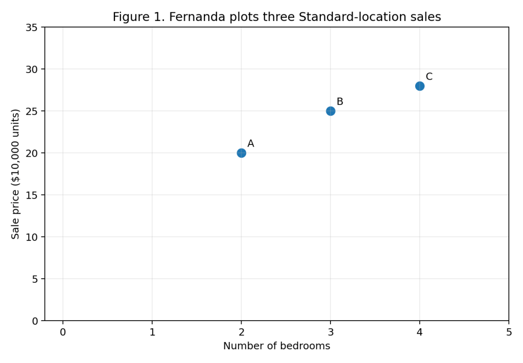
Each dot is simply one historical example. Property A tells us that one two-bedroom Standard property sold for 20 price units, or $200,000. Property B tells us that a three-bedroom Standard property sold for 25 units, and so on.
The dots seem to rise as the bedroom count rises. That does not prove anything profound about the housing universe, but it does suggest that a simple increasing relationship might be worth trying. Hmm. Interesting. Let’s continue.
4. Fernanda tries a straight-line price calculation
Fernanda notices that Property A has two bedrooms and sold for 20 units, while Property B has three bedrooms and sold for 25 units.
It appears that one extra bedroom is associated, in these two examples, with an extra 5 price units, or $50,000.
So, she tries a very simple idea:
Predicted Price = Starting Amount + (5 × Number of Bedrooms)
But what should the Starting Amount be?
For Property A, Fernanda has two bedrooms. At 5 units for each bedroom, those two bedrooms contribute the following amount:
5 × 2 = 10 units
But Property A actually sold for 20 units. So, if Fernanda wants her first calculation to get Property A exactly right, another 10 units are still needed:
Amount Still Needed to Fully Account for Property A’s Price = 20 − 10 = 10
But hang on a minute! Could Fernanda use this remaining 10 units as the amount from which her calculation starts?
In other words, before adding anything for bedrooms, could she begin with 10 units and then add the bedroom contribution on top?
If so, that gives us:
Starting Amount = Amount Still Needed to Fully Account for Property A’s Price = 10
And, therefore, Fernanda can now rewrite her earlier calculation more specifically:
Predicted Price = 10 + (5 × Number of Bedrooms)
By the way, perhaps this is a good time to attach a mathematical name to what we have just written. When two quantities are stated as being equal in this way, mathematicians call the whole statement an equation. So, from now on, we can occasionally refer to Fernanda’s calculation as her price-prediction equation. Nothing has changed in what it does. We have simply learned its mathematical name.
If you look at the above equation, you may have noticed that it does not give Fernanda just one predicted price. She can use it for any number of bedrooms. For example:
- 1 bedroom gives a predicted price of 15 units:
- Predicted Price = 10 + (5 × 1) = 10 + 5 = 15
- 2 bedrooms gives a predicted price of 20 units:
- Predicted Price = 10 + (5 × 2) = 10 + 10 = 20
- 3 bedrooms gives a predicted price of 25 units:
- Predicted Price = 10 + (5 × 3) = 10 + 15 = 25
- 4 bedrooms gives a predicted price of 30 units:
- Predicted Price = 10 + (5 × 4) = 10 + 20 = 30
Fernanda can now place these predicted prices on the same graph as the historical sale prices.
This is useful, but we need to be clear about what we are looking at. The historical points and Fernanda’s predictions are not the same thing. The historical points show what the properties actually sold for. Fernanda’s calculation shows what she would predict for a given number of bedrooms.
They can nevertheless appear on the same graph because both use the same price scale on the vertical axis.
And something rather convenient happens when Fernanda plots the prices produced by her equation: They all fall along a straight line.
If we join those predicted points, we therefore get a line showing the prices produced by Fernanda’s equation. For any bedroom count shown on the horizontal axis, the height of the line tells us the corresponding predicted price.
Now let’s put both the historical sale prices and Fernanda’s prediction line on the graph (see Figure 2 below).
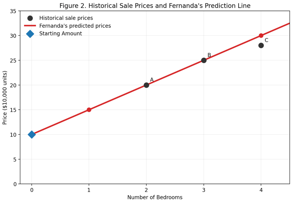
The distinction is now important (see Figure 2 above):
- The historical points show the prices at which Properties A, B and C actually sold.
- The prediction line shows the prices produced by Fernanda’s equation.
Where a historical point sits on the prediction line, Fernanda’s predicted price and the actual sale price are the same. Where it does not, her prediction differs from what actually happened.
Now look again at the number 5 in Fernanda’s equation:
Predicted Price = 10 + (5 × Number of Bedrooms)
Each time the number of bedrooms increases by one, the predicted price increases by 5 units, or $50,000. So, the number 5 controls how strongly the number of bedrooms affects the predicted price.
Next consider the number 10 in the same equation.
This is the amount from which Fernanda’s calculation starts before any bedroom contribution is added. That is why we have been calling it the Starting Amount.
We can also see this on the graph (Figure 2 above): If the Number of Bedrooms were zero, Fernanda’s calculation would give:
Predicted Price = 10 + (5 × 0) = 10
That gives us the distinctive point at 0 bedrooms and 10 price units shown on the graph.
A small warning is useful here: This does not mean Fernanda has discovered that a genuine zero-bedroom property must be worth $100,000. Zero bedrooms lies outside the little range of historical properties we are examining. The value of 10 is a setting in Fernanda’s prediction calculation (her equation). Sometimes such a starting value has a useful real-world interpretation. Then again, sometimes its main role is simply to position the prediction line appropriately.
We now understand what these parts of the calculation are doing. So, as we did in the previous article, we can attach their usual technical names:
| What We Have Just Used | Equivalent Machine Learning Term |
|---|---|
| Prices produced by Fernanda’s calculation | Predictions |
| The amount added for each additional bedroom (for example, 5) | Slope (also called a Coefficient. In later Machine Learning articles, we will encounter the related term Weight) |
| The Starting Amount (for example, 10) | Intercept (in later Machine Learning articles, we will also encounter the term Bias) |
| Fernanda’s complete price calculation (her equation) | A Linear Model |
The important point to note is that none of these names introduces a new mechanism. We have already seen what each part does. The new terminology simply gives us shorter names for ideas we now understand.
5. Two houses cooperate. The third one refuses!
Table 5 below shows Fernanda’s line prediction results so far:
| Property | Bedrooms | Predicted Price Units | Actual Price Units | Difference: Actual − Predicted |
|---|---|---|---|---|
| A | 2 | 20 | 20 | 0 |
| B | 3 | 25 | 25 | 0 |
| C | 4 | 30 | 28 | -2 |
Looking at the “Difference: Actual – Predicted” column in Table 5 above, it appears that properties A and B sit exactly on the prediction line (no error so, the line predicted the price perfectly). However, property C does not.
For C, the model predicts 30 units, or $300,000, but the house actually sold for 28 units, or $280,000. This creates the following error:
Prediction Error = Actual Price − Predicted Price = 28 − 30 = −2
The negative sign tells us that the prediction was too high by 2 units. The size of the miss is $20,000.
On the graph (see Figure 3 below), we can literally see that mistake as the vertical gap between the observed point and Fernanda’s prediction line.
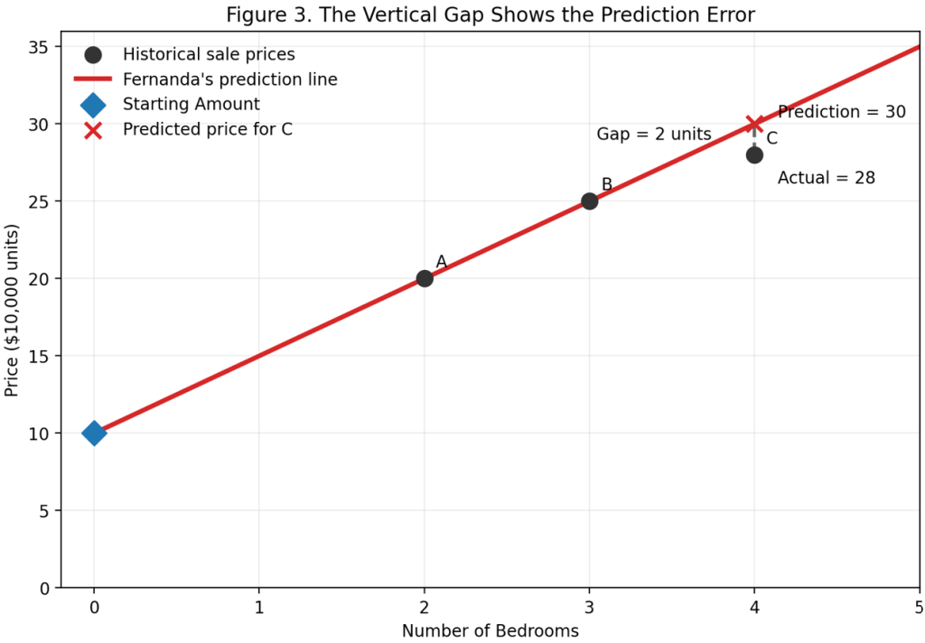
This picture is worth remembering. Later, when the mathematics becomes more compact, the basic idea will remain the same:
- The model predicts a value,
- Reality supplies the known historical value, and
- The difference tells us how far away the prediction was.
6. Which line is better?
What do you think Fernanda should do next to cater for the annoying property C that does not play ball?
Perhaps she could now move the line around. How? Well, she could change the Starting Amount. Or she could change the amount added per bedroom. Each choice would give different predictions and therefore a different line.
In any case, “I rather like the look of this line” is not a particularly convincing learning algorithm, so Fernanda needs something more robust.
In other words, she needs a consistent way to compare one possible line with another.
We already know how to measure the error for an individual property:
Prediction Error = Actual Price − Predicted Price
But Fernanda has several historical properties. So how can she combine all those individual errors into one overall measure of how well a particular line performs?
A simple first idea might be to add the errors together.
Unfortunately, that creates a problem: Positive and negative errors can cancel each other out.
Imagine one house is underestimated by $100,000 and another is overestimated by $100,000. Adding the signed errors gives zero. Declaring the model perfect at this point would be the sort of achievement best kept away from the agency’s manager!
A common solution (frequently employed by clever mathematicians) is to square each error before adding them. Squaring does two useful things for us here:
- Negative and positive errors both become positive contributions to the total, and
- Larger mistakes are penalized more strongly than smaller ones.
For Fernanda’s first line, the three errors are 0, 0 and −2. This means the total of squared errors becomes:
Total Squared Error = 0 ² + 0 ² + (−2) ² = 4
In case you were wondering, error is not a good thing, so lower is better. And since we are adding squared errors, the total cannot be negative. A total of zero, however, would mean every historical point lies exactly on the line.
7. Let another line compete
Suppose Fernanda tries another simple calculation:
Predicted Price = 12 + 4 × Number of Bedrooms
Now the three predictions are 20, 24 and 28.
| Property | Actual | First Line Prediction | Second Line Prediction |
|---|---|---|---|
| A | 20 | 20 | 20 |
| B | 25 | 25 | 24 |
| C | 28 | 30 | 28 |
The first line has squared errors 0, 0 and 4, giving a total of 4.
The second line has errors 0, 1 and 0, so its total squared error is:
Total Squared Error = 0 ² + 1 ² + 0 ² = 1
By this measure, the second line is better for these three historical examples.
Notice what has changed compared with Article 1: There we compared three complete YES/NO rules. Here we are changing numerical settings inside the same kind of calculation.
8. So where should the line go?
Fernanda now has something useful. She can propose a line, calculate its predictions, measure the individual errors and combine those errors into a single Total Squared Error.
So, in principle, she could try another line. And another. And another. But I suspect even Fernanda has better things to do with her afternoon. What she really wants is a systematic way to answer this question:
Which Starting Amount and amount added per bedroom produce the smallest Total Squared Error?
What Fernanda is trying to do here is make the model’s predictions match the historical examples as well as possible, according to the measure she has chosen.
This process is commonly called fitting the model to the data. So, when we refer to the best-fitting line, we simply mean the line whose settings give the best result according to our chosen measure. In this case, the smallest Total Squared Error.
And what we mean by a “systematic way” is this: Rather than Fernanda choosing the settings herself and then checking how well they work, could a mathematical procedure use the historical examples to determine the best settings for her?
The answer is yes.
For our three Standard-location properties, that procedure produces approximately:
Starting Amount = 12.33
Amount added per bedroom = 4
giving Fernanda the following new price-prediction calculation:
Predicted Price = 12.33 + (4 × Number of Bedrooms)
Using this new equation, Fernanda can now obtain a new set of predictions for her 3 Standard-location properties. The predictions are approximately 20.33, 24.33 and 28.33 respectively:
- Prediction for 2 bedrooms:
- 12.33 + (4 * 2) = 20.33
Prediction for 3 bedrooms:
- Prediction for 4 bedrooms:
- 12.33 + (4 * 4) = 28.33
None of the three values is exact, but the total squared error is only about 0.67:
- Prediction error for 2 bedrooms:
- 20 – 20.33 = -0.33
- Prediction error for 3 bedrooms:
- 25 – 24.33 = +0.67
- Prediction error for 4 bedrooms:
- 28 – 28.33 = -0.33
- Total Squared Error = (-0.33) 2 + (+0.67) 2 + (-0.33) 2 = 0.1089 + 0.4489 + 0.1089 = 0.6667 (approximately = 0.67)
So, compared with Fernanda’s earlier lines, this one produces a much smaller Total Squared Error.
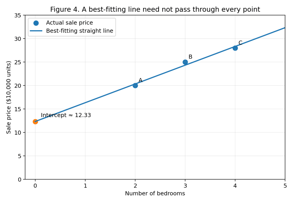
There is another interesting difference, though. None of the three historical properties now sits exactly on the prediction line. Instead, the line passes between them, leaving a small prediction error for each property.
We can see this more clearly in Figure 4 below. The historical sale prices remain as individual points, while the new prediction line is determined by:
Predicted Price = 12.33 + (4 × Number of Bedrooms)
The small vertical gaps between the historical points and the line show the remaining prediction errors.
This is an important point:
The best-fitting line does not have to pass through every historical point.
Its job is to find the straight line that performs best across the examples as a whole, according to the fitting measure we have chosen. In our case, the measure is the Total Squared Error.
We are not yet going to derive the mathematics that produces the values 12.33 and 4. That is not because the mathematics is forbidden territory. Quite the opposite. Our immediate objective is to understand what the procedure is trying to achieve before worrying about how it finds those values.
For now, the arithmetic above is enough to verify that these settings give us a substantially smaller Total Squared Error than the alternatives we tried earlier.
And now we can finally attach a name to what we have just done.
We started with historical examples, used their prediction errors to judge different settings, and found the settings that make our linear model fit those examples as well as possible according to our chosen criterion.
This process of fitting a linear model to numerical data is called Linear Regression.
9. Location has not mysteriously disappeared
So far, Fernanda has deliberately held location fixed by looking only at Standard properties. That made the first graph easy to understand.
But our real task uses both Bedrooms and Location. We therefore need a way to include location in the same calculation. But how best can she do this?
Fernanda notes that Bedrooms are already numerical, so she can multiply the number of bedrooms by a chosen amount and add that contribution to the Starting Amount. However, location is different: Standard and Prime are words, not numbers.
If Fernanda wants to include Location in the same kind of calculation, she first needs a numerical way to represent those two possibilities.
One simple choice is as shown in Table 7 below:
| Location | Location Code |
|---|---|
| Standard | 0 |
| Prime | 1 |
This does not mean Standard is “worth zero” and Prime is “worth one”. The numbers are being used as a form of switch, to easily differentiate between the two.
If the Location Code is 0, the extra Prime-location contribution is switched off (meaning the location is Standard).
If the Location Code is 1, that contribution is included (meaning the location is Prime).
Armed with this new technique (thanks to mathematicians again), Fernanda now proposes a three-part equation:
Predicted Price = Starting Amount + (Bedroom Contribution × Bedrooms) + (Location Contribution × Location Code)
Note that in Machine Learning, these adjustable contributions are often controlled by numbers called weights (or coefficients in Linear Regression). So, later, we may refer to the Bedroom Contribution and Location Contribution as the Bedroom Weight and Location Weight.
In the above equation:
- The Bedroom Contribution controls how much the predicted price changes when Bedrooms increases by one, while Location is kept fixed,
- The Location Contribution controls how much the predicted price changes when we move from Standard to Prime, while Bedrooms is kept fixed.
10. Fernanda’s first complete two-input model
Let us begin with settings that are easy to understand and easy to calculate:
- Starting Amount = 10
- Bedroom Weight = 5
- Location Weight = 10
So, assuming Fernanda chooses these values, her first full calculation will be:
Predicted Price = 10 + (5 × Bedrooms) + (10 × Location Code)
For a two-bedroom Prime property, the calculation generates:
Predicted Price = 10 + (5 × 2) + (10 × 1) = 30
That means the predicted price is estimated as $300,000.
Similarly, for a four-bedroom Standard property we have:
Predicted Price = 10 + (5 × 4) + (10 × 0) = 30
Again, resulting in $300,000. Here, the Prime contribution disappeared because its Location Code is zero.
11. Let us test those settings against all six houses
Applying the new equation to the 6 historical cases, we get a new set of predictions to compare against the actual sale values (see Table 8 below):
| Property | Bedrooms | Location Code | Actual | Predicted | Error |
|---|---|---|---|---|---|
| A | 2 | 0 | 20 | 20 | 0 |
| B | 3 | 0 | 25 | 25 | 0 |
| C | 4 | 0 | 28 | 30 | -2 |
| D | 2 | 1 | 30 | 30 | 0 |
| E | 3 | 1 | 40 | 35 | 5 |
| F | 4 | 1 | 45 | 40 | 5 |
This model is not disastrous. It even gets three of the six prices exactly right in our artificial little world.
But exact hits are not the right way to judge a continuous price prediction. The three misses have different sizes, and that information matters.
Using the squared-error approach, the score is:
Total Squared Error = 0 ² + 0 ² + (−2) ² + 0 ² + 5 ² + 5 ² = 54
That gives us one number with which to compare another set of settings.
12. Learning now means changing numerical settings
Suppose the learning procedure keeps the same form of calculation but changes the numbers inside it.
For example, if it increases the Location Weight from 10 to 13 while leaving the other two settings unchanged, we get:
Predicted Price = 10 + (5 × Bedrooms) + (13 × Location Code)
The new predictions are 20, 25, 30, 33, 38 and 43.
If you get some time, try and reproduce Table 8 entries with the new settings. This will be a short but good exercise to complete and will help you gain a little more confidence in this type of activity.
Using the new set of predictions, the corresponding errors are 0, 0, −2, −3, 2 and 2, resulting in:
Total Squared Error = 0 ² + 0 ² + (−2) ² + (-3) ² + 2 ² + 2 ² = 21
The new Total Squared Error is clearly a substantial improvement from 54.
This is the central learning idea in this article:
Keep the general prediction structure, use historical examples to assess its performance, and change the numerical settings to improve the fit.
Of course, a real Linear Regression procedure does not normally sit there trying random numbers with Fernanda cheering whenever the score falls. There are systematic mathematical ways to find the settings that minimize the chosen error measure.
We will go deeper into how learning algorithms decide which settings to change, and by how much, later in this series. For now, it is enough to see what is being adjusted and what makes one set of settings better than another.
13. What settings does Linear Regression choose for all six houses?
In the previous section, Fernanda improved the model by changing just one setting: The Location Contribution. That reduced the Total Squared Error from 54 to 21.
But our complete two-input model has three adjustable settings:
- the Starting Amount,
- the Bedroom Contribution, and
- the Location Contribution.
There is no particular reason why Fernanda should change only one of them while leaving the other two untouched.
So, instead of adjusting the settings manually, we can now use the same fitting process we introduced earlier and ask a broader question:
Which combination of all three settings gives the smallest Total Squared Error across all six historical properties?
Using Bedrooms and Location Code as the two inputs, Linear Regression gives approximately:
- Starting Amount = 7.08
- Bedroom Weight = 5.75
- Location Weight = 14.00
Note: Later in this series, we will see one important way a learning procedure can work out how numerical settings should change. For now, you will have to take my word for these three values. Fortunately, my word is gold😊!
Using the above settings, Fernanda’s fitted two-input model therefore becomes:
Predicted Price = 7.08 + (5.75 × Bedrooms) + (14 × Location Code)
Let us now see what this model predicts for all six historical properties (see Table 9 below):
| Property | Actual Price Units | Predicted Price Units | Approx. Predicted Dollars |
|---|---|---|---|
| A | 20 | 18.58 | $185,800 |
| B | 25 | 24.33 | $243,300 |
| C | 28 | 30.08 | $300,800 |
| D | 30 | 32.58 | $325,800 |
| E | 40 | 38.33 | $383,300 |
| F | 45 | 44.08 | $440,800 |
The Total Squared Error is now approximately 17.08:
Total Squared Error = (20 – 18.58) 2 + (25 – 24.33) 2 + (28 – 30.08) 2 + (30 – 32.58) 2 + (40 – 38.33) 2 + (45 – 44.08) 2 = 17.0834 (approximately 17.08)
So, the progression has been:
- 54 with Fernanda’s first complete set of settings,
- 21 after manually improving one setting,
- 17.08 after Linear Regression adjusts all three settings together.
That is the important point: Linear Regression is not trying to make one or two houses come out perfectly. It is trying to find the combination of settings that performs best across all six historical properties together, according to the measure we chose: Total Squared Error.
And please do not be disturbed by predictions such as $243,300 (property B). A mathematical model is perfectly happy to produce a number that an estate agent might consider slightly awkward for a glossy brochure!
Also notice that the fitted model does not reproduce every historical sale price exactly. That is not a failure. It is balancing the errors across all six examples while staying within the simple linear model we gave it.
One final point is worth stressing here: Linear Regression did not decide that Bedrooms and Location were the right inputs to use. We supplied those inputs. It also did not invent the structure of Fernanda’s equation. We supplied that too.
What it determined from the historical examples were the numerical settings inside that model:
7.08, 5.75 and 14.00.
That is the learning taking place here.
14. What exactly has been learned?
This is worth being precise about because the word “learned” is easily asked to do too much work.
In our example, people decided:
- The question: predict sale price,
- The inputs available to the model: Bedrooms and Location,
- How Location would be represented numerically: 0, 1 instead of Standard and Prime,
- The general form of the calculation: Starting Amount plus a contribution from each input,
- Which historical examples would be used: Our 6 examples,
- That squared prediction errors would be used to judge the fit: Total Squared Error.
The learning procedure used those examples to determine the numerical settings that best satisfy that criterion. It did not independently discover that Bedrooms and Location are the only important facts about a house. We gave it those inputs.
It did not understand that Prime locations contain better cafés, nicer parks or more persuasive estate-agent adjectives!
And it did not reason like Fernanda.
The human story helps us understand the mechanism. The algorithm itself manipulates numerical inputs and numerical settings according to a specified procedure.
15. Time to attach the technical names
We have now used most of the important ingredients of a simple Linear Regression model. Let us attach their usual names (see Table 10 below):
| What We Have Been Using | Usual Technical Name |
|---|---|
| Bedrooms and Location Code | Inputs or Features |
| The known Actual Sale Price used during fitting | Target or known Output |
| Actual Price − Predicted Price | Prediction Error (often called a Residual in regression) |
| Adding the squared prediction errors across the historical examples | Total Squared Error (our chosen fitting measure) |
| The numerical values determined from the historical examples, such as 7.08, 5.75 and 14 | Fitted Settings or Model Parameters |
| Fernanda’s complete equation after those settings have been determined | Fitted Linear Model |
At this point, the name Linear Regression should hopefully feel a little less mysterious. We can now see where both parts of the name come from:
- Regression: In our example, we are predicting a numerical value (the sale price), rather than a YES/NO category,
- Linear: Our predicted price is produced by starting with an intercept (Starting Amount) and then adding a contribution from each input. Each contribution is calculated by multiplying the input by its coefficient (or weight).
With only Bedrooms as an input, this relationship appeared as the straight line we could see on our graph. With Bedrooms and Location together, the same basic idea continues even though it is no longer as convenient to show on a simple two-dimensional graph.
16. How mathematicians write the same calculation
So far, we have deliberately used proper names in our equations. They make it easier to see what each quantity means.
However, mathematicians and Machine Learning texts usually compress the same idea into symbols. For example, our two-input calculation may be written as:
Predicted Price = Bias + Bedroom Weight × Bedrooms + Location Weight × Location
and then shortened to something like:
ŷ = b + w₁x₁ + w₂x₂
where:
- ŷ means the predicted output,
- b is the bias or intercept,
- w₁ is the weight attached to the first input,
- x₁ is the first input value,
- w2 is the weight attached to the second input,
- x2 is the second input value.
Nothing new has happened mathematically. The notation is simply shorter.
This is a useful discipline throughout the series: Understand the mechanism first, then let notation save space rather than create mystery.
17. But where did our nice straight line go?
With one numerical input, such as Bedrooms alone, the model can be shown as an ordinary straight line on a two-dimensional graph.
With two numerical inputs, the geometry extends to a flat surface rather than a single line on a page. With still more inputs, the same linear idea continues into dimensions that are less convenient to draw and rather less useful for decorating a blog post (I like my readers but there is a limit to how far I am willing to go to satisfy their curiosity).
The important point is that the model remains linear in its input contributions:
Start with the bias, multiply each input by its weight, and add the contributions.
So, the graph was not a childish simplification that we now throw away. It showed the one-input version of the same mechanism.
18. A new house arrives
Life is never easy though.
Suppose Fernanda receives another three-bedroom property in a Prime location.
Using the fitted settings she gets:
Predicted Price = 7.08 + 5.75 × 3 + 14 × 1
Predicted Price = 38.33 price units ≈ $383,300
Notice something slightly uncomfortable but important. Property E in our historical data also had three bedrooms and a Prime location. Our model therefore gives the new property exactly the same prediction.
That is not because the two houses are identical. It is because, as far as this model is concerned, they are identical: After all, Bedrooms and Location are the only inputs it receives.
If the new house has a leaking roof, a spectacular terrace or a nightclub masquerading as “local vibrancy”, the model knows none of that unless we supply additional information.
19. Does the Bedroom Weight tell us what a bedroom is worth?
Hmm. Not quite.
In this fitted model, the Bedroom Weight is 5.75 price units. It is tempting to translate that directly as “an extra bedroom is worth $57,500”.
A more careful statement would be:
Holding the Location Code fixed, this model increases its predicted price by $57,500 when the bedroom count increases by one.
That is a statement about the model’s prediction, not automatically a causal fact about the real world. For example, perhaps larger homes tend to have more bedrooms. Or perhaps certain neighborhoods have both larger houses and higher prices. Or perhaps our six examples are simply too small to support grand declarations about property economics.
Linear Regression can reveal predictive relationships. Establishing that changing one feature would cause the outcome to change by a particular amount is a different question, which we will tackle later in this series.
20. Is Linear Regression too simple to matter?
Nope.
A simple method can be useful because it is understandable, quick to compute and easy to inspect. In some problems a linear relationship is genuinely a good approximation. In others it provides a useful baseline against which more complicated methods can be judged.
Its limitations, however, are equally important:
- The model can use only the inputs we provide,
- It assumes the input contributions combine in the specified linear way,
- Unusual cases may be badly predicted,
- A good fit to historical examples does not guarantee good predictions on new properties,
- The fitted weights describe the model and data. They should not automatically be treated as causal effects.
In other words, Linear Regression is neither magic nor merely a classroom toy. It is a precise tool with assumptions, strengths and limits. Use it wisely!
21. Question time
Before moving on, consider the following:
- In our full model, what are the inputs and what is the output?
- If the Bedroom Weight increases while everything else stays fixed, what happens to the predicted price of a four-bedroom property?
- Why is the Starting Amount also called the intercept?
- Why can “simply adding signed prediction errors” be misleading?
- Did the learning procedure discover that Location should be an input, or did people make that choice?
- If two properties have the same Bedrooms and Location Code but differ greatly in condition, what will this model do?
22. What have we learned?
Fernanda began with a new kind of question. Instead of predicting a YES/NO category, she needed to predict an actual price.
We first isolated one input and drew historical examples on a graph. That let us see how a straight-line prediction combines:
- A Starting Amount, which appears as the intercept, and
- An input contribution controlled by a weight.
We then saw that historical points do not generally sit perfectly on one line. The vertical gaps between actual values and predictions are prediction errors.
To compare possible lines and settings, we squared those errors and added them. This gave us a single number to minimize.
We then brought Location back into the model, represented it numerically, and saw that learning can mean changing several numerical settings rather than choosing among a few complete rules.
Most importantly, we learned that:
- The prediction combines a bias/intercept with a contribution from each input,
- The weights and bias are adjustable settings,
- Historical examples allow a learning procedure to choose settings that reduce prediction error,
- The best-fitting model need not reproduce every historical example exactly,
- The human analogy explains the mechanism and illustrates the kind of numerical calculations the algorithm performs,
- A fitted weight describes the model’s predictive relationship and is not automatically a causal statement.
We have therefore moved one step beyond Article 1.
There, learning selected which complete rule to use. Here, learning selected numerical settings inside a prediction calculation.
23. Next: What if Fernanda only needs YES or NO again?
What? “You must be joking”, I hear you say!
Sadly, I am not. After all this effort to predict an actual price, we are going back to a familiar question:
Is this property expected to sell for at least $300,000: YES or NO?
And you would be perfectly entitled to ask two questions.
First: Didn’t we already do this in Article 1?
Yes. But there we approached the problem by giving the computer several complete YES/NO rules and asking it to choose the one that worked best.
Second: Couldn’t we simply use the price prediction from this article and check whether it is at least $300,000?
Absolutely. And for our little property example, that would be perfectly reasonable. We do not actually need another mechanism just to answer this particular question.
However, many real problems ask directly for a decision rather than for a numerical quantity first, including YES or NO, approve or reject, fraud or legitimate, and so on. In such cases, it can be useful to build the decision directly from the available inputs.
That is what we are going to explore next. The inputs will contribute to a numerical score, and we will ask whether that score crosses a cutoff.
There is another reason for taking this apparent detour: This simple mechanism turns out to be an important stepping stone toward something much more powerful: The artificial neuron and, eventually, Neural Networks.
So, we are not returning to YES/NO because Article 1 failed. We are returning to it because we are now ready to understand a different mechanism for producing that decision.
24. Question time: Suggested answers
Here are some answers to the questions posed in section 21 above:
- Bedrooms and Location Code are the inputs. The output is Predicted Sale Price.
- The prediction rises. The increase equals the change in Bedroom Weight multiplied by four, because that property has four bedrooms.
- With one input, the Starting Amount is the value where the prediction line crosses the vertical axis, which occurs when the input value is zero.
- Positive and negative errors can cancel. A large overprediction and a large underprediction can therefore misleadingly sum to zero.
- People chose to provide Location as an input. The learning procedure adjusted the numerical setting attached to it.
- It gives them the same prediction because, from the model’s point of view, the supplied inputs are identical. Condition is invisible to this model.
Feedback please 😊

